I’m happy to announce a new set of features for our tool Bio4jExplorer plus some changes in its design. I hope this may help both potential and current users to get a better understanding of Bio4j DB structure and contents.
Node & Relationship properties
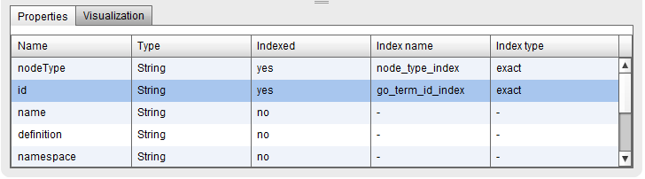
You can now check with Bio4jExplorer the properties that has either a node or relationship in the table situated on the lower part of the interface. Five columns are included:
Name: property name
Type: property type (String, int, float, String[], …)
Indexed: either the property is indexed or not (yes/no)
Index name: name of the index associated to this property -if there’s any
Index name: type of the index associated to this property -if there’s any
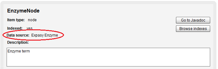
Node & Relationship Data source
You can also see now from which source a Node or Relationship was imported, some examples would be Uniprot, Uniref, GO, RefSeq…
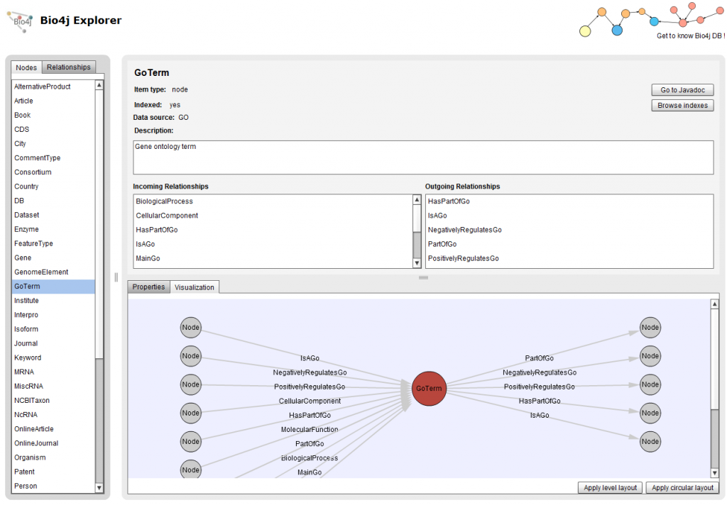
Relationships Name property
With this new version you can directly check here the “internal” name of relationships without having to go to the respective javadoc documentation.
This is quite useful when you are writing your Cypher or Gremlin queries, just check it, copy it, and paste it in your query. An example using the relationship shown in the picture would be this query included in the Bio4j Cypher cheatsheet:
Get proteins (accession and names) associated to an interpro motif (limited to 10 results)
12345
>
START i=node:interpro_id_index(interpro_id_index = "IPR023306")
 MATCH i <-[:**PROTEIN_INTERPRO**]- p
 return p.accession, p.fullname, p.name, p.short_name
 limit 10
In case you are interested on how the tool is implemented, please go to the previous post about Bio4jExplorer where you can find information about the different code repos and more info.
If you want to check the files including the hard-coded information regarding how nodes, relationships, and indexes are organized, and which is the input for the program which creates the AWS SimpleDB domain, I just uploaded them to the bio4j-public S3 bucket. Please click on their names to download them:
There have already been a good few posts showing different uses and applications of Bio4j, but what about Bio4j data itself?
Today I’m going to show you some basic statistics about the different types of nodes and relationships Bio4j is made up of.
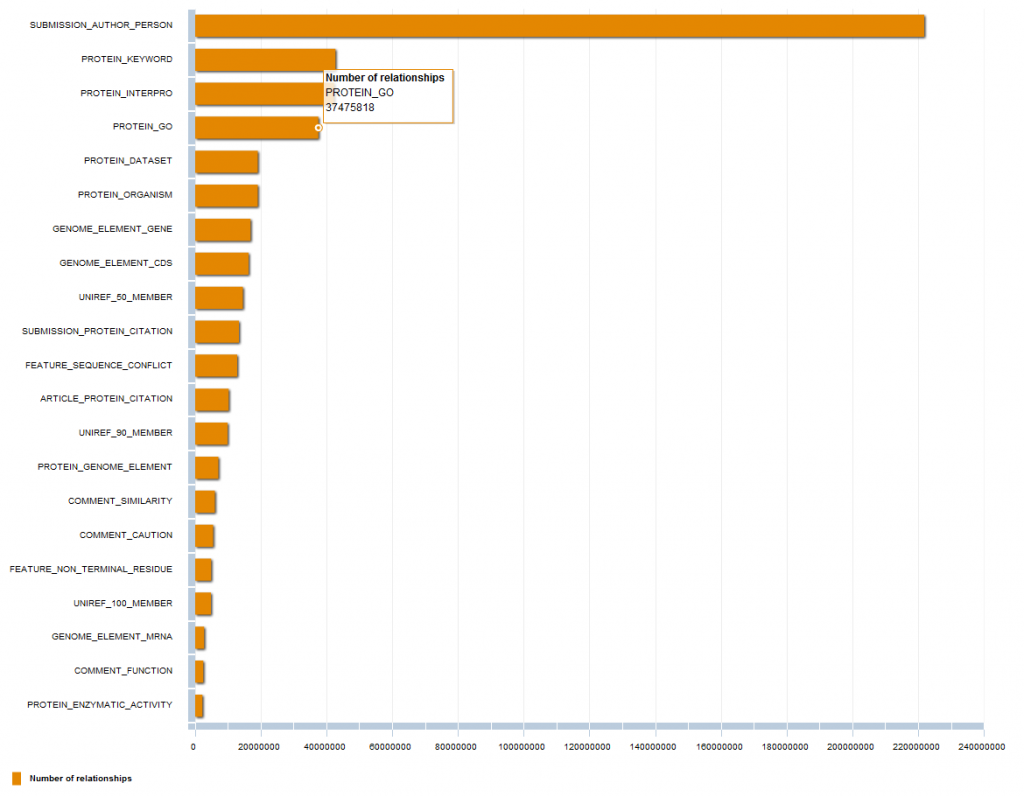
Just as a heads up, here are the general numbers of Bio4j 0.7 :
Number of Relationships: 530.642.683
Number of Nodes: 76.071.411
Relationship types: 139
Node types: 38
Ok, but how are those relationships and nodes distributed among the different types? In this chart you can see the first 20 Relationship types (click on the image below to check the interactive chart):
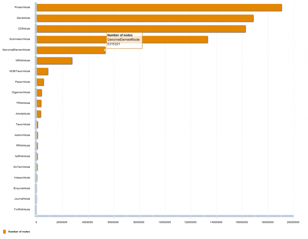
Here, the same thing but for the first 20 Node types (click on the image below to check the interactive chart):
You can also check these two files including the numbers from all existing types:
Patrick Durusau
Excellent!
Question: When I checked at PubMed, I did not find Neo4j cited in any of the medical literature. I am not a medical professional but am interested in what might promote Bio4j in the medical research community?
It is too good of a resource to be unnoticed.
Patrick
ppareja
Hi Patrick,
I’m glad you liked the post.
It’s true that Bio4j may not have caught the attention of many people yet who could definitely make a good use out of it. What are the reasons for that? Well, I think it could be a mixture of factors.
Some people don’t like too much learning new technologies/strategies/workflows… and tend to stick to things they already know as long as possible – which is totally respectable and undestandable. Other people though, may simply not have found about it yet… It’s also possible that due to the lack of a well structured project documentation, potential users get lost in their way when trying to figure out what’s Bio4j about and/or miss the parts they could be interested in.
I could keep on going with more possible reasons that are coming to my mind but still, couldn’t be really objective – it’s me who created this project :D
The point you bring up is actually one of the reasons why we value so much any sort of feedback for the project, (specially constructive ‘bad’ feedback that help us realize its weaknesses)
Let me know if you come up with an idea to let more people know about Bio4j !
Pablo
If that’s what you’re thinking, please go here to get an idea of what’s this all about.
From now on, this CloudFormation template adapts the server configuration files:
neo4j-wrapper.conf
neo4j.properties
to the characteristics of the instance type the server is running in, so that it can make the best out of it.
These configurations assume that the server is running alone in the machine.
For that I created these two new mappings in the template:
AWSInstanceType2WrapperConfFile
AWSInstanceType2Neo4jPropertiesFile
Default configuration values are available in the bio4j-public S3 bucket. For example in order to have access to the server configuration files of a m1.xlarge instance, just go to this url:
I don’t know if you have ever heard of the lowest common ancestor problem in graph theory and computer science but it’s actually pretty simple. As its name says, it consists of finding the common ancestor for two different nodes which has the lowest level possible in the tree/graph.
Even though it is normally defined for only two nodes given it can easily be extended for a set of nodes with an arbitrary size. This is a quite common scenario that can be found across multiple fields and **taxonomy **is one of them.
The reason I’m talking about all this is because today I ran into the need to make use of such algorithm as part of some improvements in our metagenomicsMG7 method. After doing some research looking for existing solutions, I came to the conclusion that I should implement my own, I couldn’t find any applicable implementation that was thought for more than just two nodes.
Ok, but let’s get into detail and see my algorithm:
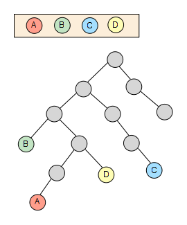
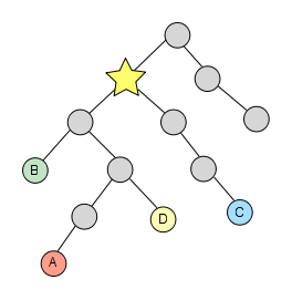
We start from a set of nodes with an arbitrary length -4 in this sample, which are spread through the taxonomy tree:
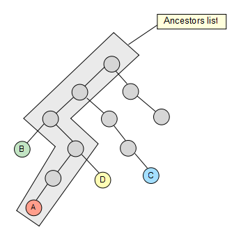
We fetch then the first node from the set and calculate its whole ancestor list to the main root of the taxonomy.
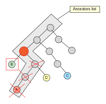
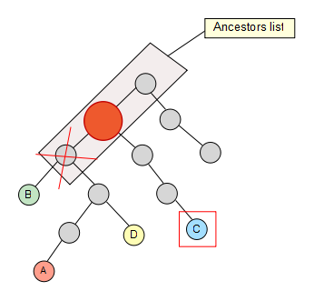
Now that we have the list, we take the second node of the set and check if it’s contained in it, if not, we keep going up through its ancestors until we find a hit. Once the hit has been found, we get rid of the previous elements in the list (if any) so that they are not taken into account for the next iterations in the algorithm.
We keep going trough our node set, and C also removes some elements of the list…
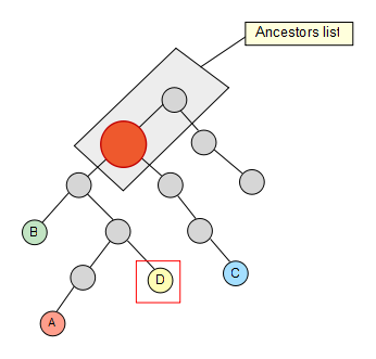
Finally we reach the last node of our set, but no element is removed from our list as a result.
The last thing we have to do is simply get the first element of the resulting list and there we have our lowest common ancestor!
This algorithm is encapsulated in the class TaxonomyAlgo, specifically in the static method lowestCommonAncestor() that expects a list of NCBITaxonNode as parameter and returns their LCA node.
You can also check the class LowestCommonAncestorTest where a simple test program that makes use of this method is implemented.
This program expects as parameters:
Bio4j DB folder
An arbitrary number of NCBI taxonomy IDs representing the node set
The Scientific name and the NCBI tax ID of the LCA are printed in the console as result.
Paul Agapow
Oddly enough, I had to solve this exact problem a few years ago (to see how much of a tree is left after an extinction, for calculating the biodiversity impact) and then just a few weeks ago (but for the unrooted case). Both times I was sure this had to be a solved problem, but there were no obvious solution out there.
Pablo Pareja
Hi Paul,
I was also quite surprised there wasn’t any ‘official’/obvious solution for this, specially when I’d say it’s quite a common problem.
Now that you mention it, I think I’ll extend the implementation for the unrooted case as well.
By the way, just out of curiosity, what kind of solution did you come up with in the end?
Victor de Jager
Hi Pablo,
interesting post. I solved a very similar problem a few years ago using an early version of the ETE toolkit. http://ete.cgenomics.org/
It’s a well documented with plenty of examples.
ppareja
Hi Victor,
Thanks for the link. Just a quick question, is it open-source?
Jaime
Hi,
You may be interested in this python script based on the ETE library: https://github.com/jhcepas/ncbi_taxonomy
BTW, ETE is free software
Miguel
The LCA problem is closely related to the Range Minimum Query problem in graph theory. Working on metagenomics I had to implement a fast algorithm to search for LCA of an arbitrary number of leafs in a taxonomic tree. Given that the tree is always the same, you can pre-process it for fast searches. I ended up implemented the Sparse table algorithm for RMQ explained here:
[](http://community.topcoder.com/tc?module=Static&d1=tutorials&d2=lowestCommonAncestor)
You say in your post that you couldn’t find any solution out there for more than 2 nodes. The reason is simple: the LCA of N nodes can be decomposed to N-1 times the LCAs of 2 nodes (for example, the LCA of 3 nodes is the LCA of one of them and the LCA of the other 2).
ppareja
Hi Miguel,
Thanks for the link ;)
In my case though I didn’t want to do any pre-processing on purpose. Having everything stored as a graph gives you a great advantage both in terms of speed and scalability and I didn’t want to throw that away. On the other hand this sort of algorithm is one that could be applied to other sub-graphs of Bio4j, not only the taxonomy tree, so once you implement it in this way it’d be trivial to adapt it to other such cases.
I know that the problem can be decomposed so that you end up with a set of 2-nodes problems, what I meant however was that I expected to find algorithms for this problem with some sort of specific optimizations when dealing with a big set of nodes, not only two. For example somehow not passing again through nodes already visited, which will happen when you do decomposing the problem in “isolated” pairs of nodes.
After writing this post on December, I’ve been thinking of doing something similar, yet different, using Neo4j Cypher query language.
That’s where I came up with the idea of looking for topological patterns through a large sub-set of the Protein-Protein interactions network included in Bio4j; -rather than focusing in a few proteins selected a priori.
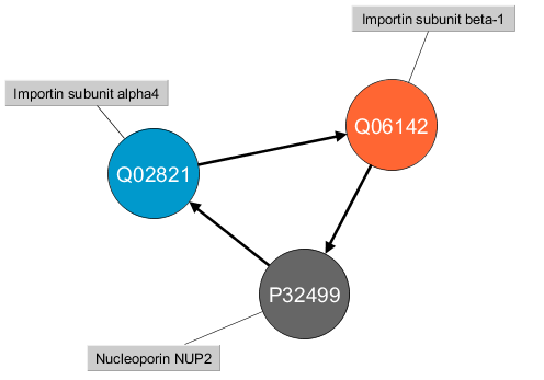
I decided to mine the data in order to find circuits/simple cycles of length 3 where at least one protein is from Swiss-Prot dataset:
I would like to point out that the direction here is important and these two cycles:
A --> B --> C --> A
A --> C --> B --> A
are not the same. Ok, so once this has been said, let’s see how the Cypher query looks like:
As you can see it’s really simple and straightforward. In the first two lines we match the proteins from Swiss-Prot dataset for later retrieving the ones which form a 3-length cycle as described before. Once the query has finished, you should be getting something like this:
As you can see the query took about 17 minutes to be completed in a 100% fresh DB -there was no information cached at all yet; with a m1.large AWS machine -this machine has 7.5GB of RAM.
Not bad, right!?
We have to beware of something though, this query returns cycles such as:
A --> B --> C --> A
B --> C --> A --> B
as different cycles when they are actually not. That’s why I developed a simple program to remove these repetitions as well as for fetching some statistics information.
After running the program you get two files:
PPICircuitsLength3NoRepeats file: download it here
The final circuits found were reduced after performing the filtering to 2226 records.
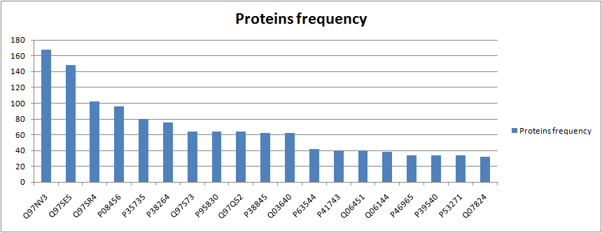
Finally, I also created a really simple chart including the absolute frequency of the first 20 proteins with more occurrences in the cycles that were found.
All properties found have been incorporated to the enzyme node including:
ID
Official name
Alternate names
Cofactors
Comments
Catalytic activity
Prosite cross-references
Node type indexing
From now on, every node present in the database has a property nodeType including its type which has been indexed. That way you can now access all nodes belonging to an specific type really easily.
Availability in all Regions
The AWS region you are based in won’t be a problem for using Bio4j anymore. EBS Snapshots have been created in all regions as well as CloudFormation templates have been updated so that they can now be used regardless the region where you want to create the stack.
Only Asia Pacific (Singapore) ap-southeast-1 region is not ready due to ongoing issues from AWS side regarding extremely slow S3 object downloading. Hope we can find a work around for this soon!
New CloudFormation templates
Basic Bio4j instance (updated)
The basic Bio4j instance template has been updated so that now you can use it from all zones. Check out more info about this in the updated blog post
Basic Bio4j REST server
A new template has been developed so that you can easily deploy your Neo4j-Bio4j REST server in less than a minute.
This template is available in the following address:
The steps you should follow to create the stack are really simple. Actually, you can follow as a guide this blog post about the template I created for deploying a general Neo4j server, only one or two parameters vary
Bio4j REST server
Once you get your server running thanks to the useful template I just mentioned before, using Neo4j WebAdmin with Bio4j as source you will be able to:
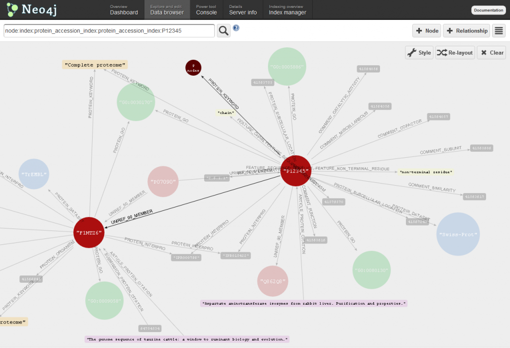
Explore you database with the Data browser
Using the data browser tab of the Web administration tool you can explore in real-time the contents of Bio4j!
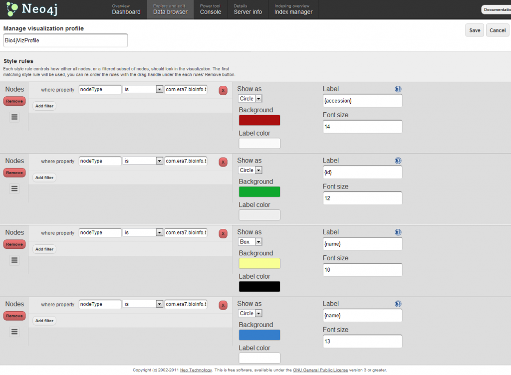
In order to get visualizations like the one shown above, you should make use of visualization profiles. There you can specify different styles associated to customizable rules which can be expressed in terms of the node properties. Here’s a screenshot showing how the visualization profile I used for the visualization above looks like:
Just beware of one thing, the behavior of the tool is such that it does not distinguish between highly connected nodes and more isolated ones. Because of this, clicking nodes such as Trembl dataset node is not advisable unless you want to see it freeze forever -this node has more than 15 million relationships linking it to proteins.
Run queries with Cypher
Cypher what?!
Cypher **is a **declarative language which allows for expressive and efficient querying of the graph store without having to write traversers in code. It focuses on the clarity of expressing what to retrieve from a graph, not how to do it, in contrast to imperative languages like Java, and scripting languages like Gremlin.
A query to retrieve protein interaction circuits of length 3 with proteins belonging to Swiss-Prot dataset (limited to 5 results) would look like this in Cypher:
If you want to check out more examples of Bio4j + Cypher, check our Bio4j cypher cheat sheet that we will be updating from time to time.
Querying Bio4j with Gremlin
Gremlins? What do they have to do with Bio4j!?
Gremlin is a graph traversal language that can be natively used in various JVM languages - it currently provides native support for Java, Groovy, and Scala. However, it can express in a few lines of code what it would take many, many lines of code in Java to express.
Querying proteins associated to the interpro motif with id IPR023306 in Bio4j with Gremlin would look like this: (limited to 5 results)
If you want to check out more examples of Bio4j + Gremlin, check our Bio4j gremlin cheat sheet that we will be updating from time to time.
Bug fixes
Dataset nodes There was a bug in the importing process which resulted in the creation of a new dataset node everytime a new Uniprot entry was stored. Now everything’s fine!
So that’s all for now! Hope you enjoy all this changes and new features I’ve been working on in the last couple of months. As always, feel free to give any feedback you may have, I’m looking forward to it ;)
Today I managed to find some time to check out the Graph-algo component from Neo4j and after playing with it plus Bio4j a bit, I have to say it seems pretty cool.
For those who don’t know what I’m talking about, here you have the description you can find in Neo4j wiki:
This is a component that offers implementations of common graph algorithms on top of Neo4j. It is mostly focused around finding paths, like finding the shortest path between two nodes, but it also contains a few different centrality measures, like betweenness centrality for nodes.
The algorithm for finding the shortest path between two nodes caught my attention and I started to wonder how could I give it a try applying it to the data included in Bio4j. I realized then that protein-protein interactions could be a good candidate so I got down to work and created the utility method:
findShortestInteractionPath(ProteinNode proteinSource, ProteinNode proteinTarget, int maxDepth, int maxResultsNumber)
for getting at most maxResultsNumber paths between proteinSource and proteinTarget with a maximum path depth of maxDepth.
You can check the source code here
I also did a small test program which prints out the paths found between two proteins.
Even though I’ve missed having a wider choice of algorithms, it’s really cool having at least this small set of algorithms already implemented, abstracting you from the low level coding.
Apart from that, I’ve been thinking how Bio4j could open a lot of doors for topology/network analysis around all the data it includes. Such analysis could otherwise be quite hard to perform due to several reasons like the lack of data-integration between different datasources and the inner storage paradigm limiting topology/network analysis among others…
With Bio4j however, you just have to move around the nodes and get the information you’re looking for! ;)
alper yilmaz
it’s getting more interesting.. :)
that’s what I meant by “data-mining” during our skype conference.. cool..
Roji
I follow neo4j which much itrneest. It is a novel approach, however i think property searches are very important and neo4j is not very good at this.So for example, implementing a complete social website with millions of users would not be feasible with neo4j i think. I am not sure off course.What is also itrneesting is the upcoming of native XML database. They also solve the imdependace mismatch to a certain expend. However their model are trees not graphs, graphs are more general in this sense, but i think more optimizations are possible if you choose trees.
ppareja
Hi Roji,
Could you provide some reasons why you think property searches are not good with Neo4j?
Regarding XML databases and other tree-oriented options, they definitely are great for many use cases, however when you have to deal with highly connected data they may not be enough. The case depicted in this blog post is a good example, even just modelling protein-protein interactions would not be possible with a tree – you get plenty of cycles which cannot be expressed with that paradigm…
UPDATE: You can now use this template from **all zones but ap-southeast-1! **
Hi!
So this week it was time to finally start using CloudFormation together with Bio4j. For those not familiar with this AWS service, quoting from their site:
AWS CloudFormation gives developers and systems administrators an easy way to create and manage a collection of related AWS resources, provisioning and updating them in an orderly and predictable fashion.
This is really useful because thanks to CloudFormation templates, you don’t have to worry about manually launching an instance, create a volume, attach it, do some stuff, and then free the resources… You can encapsulate all this tasks in a template reducing all the tasks to just two:
**create **the stack
**delete **the satck whenever you are done with it
This template is available in the following address:
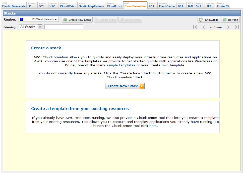
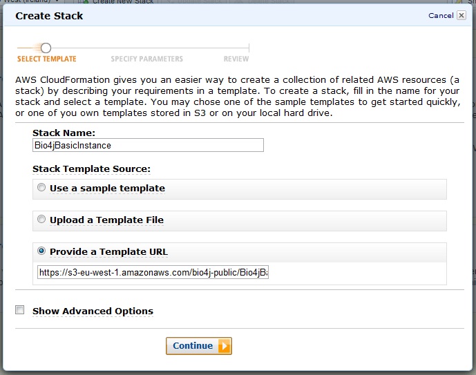
So, let’s see how easy it actually is to create your stack. First you should go to the CloudFormation tab in the amazon console and click the button: Create New Stack:
You will see this new window now where you should choose the option Provide a template URL’ and paste there the URL I just provided before. You should also give your stack a name filling the field Stack name. Then click Continue.
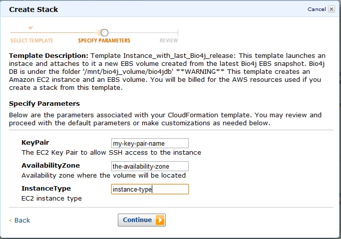
Ok, now you should be seeing this:
Provide then your key-pair name, availability zone, and finally enter the type of instance you want to launch.
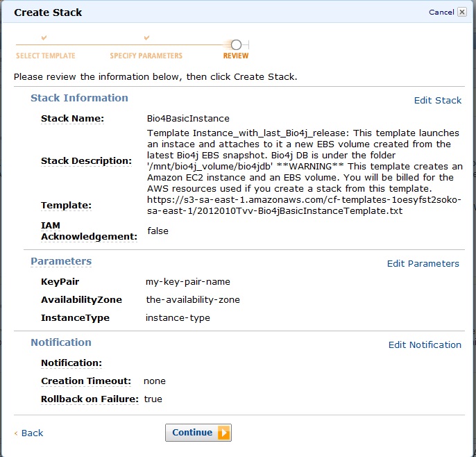
Once you clicked continue you’ll see a review of all the parameters you entered so far like:
Check everything is as you wish and click continue.
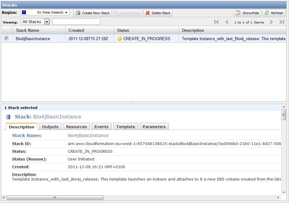
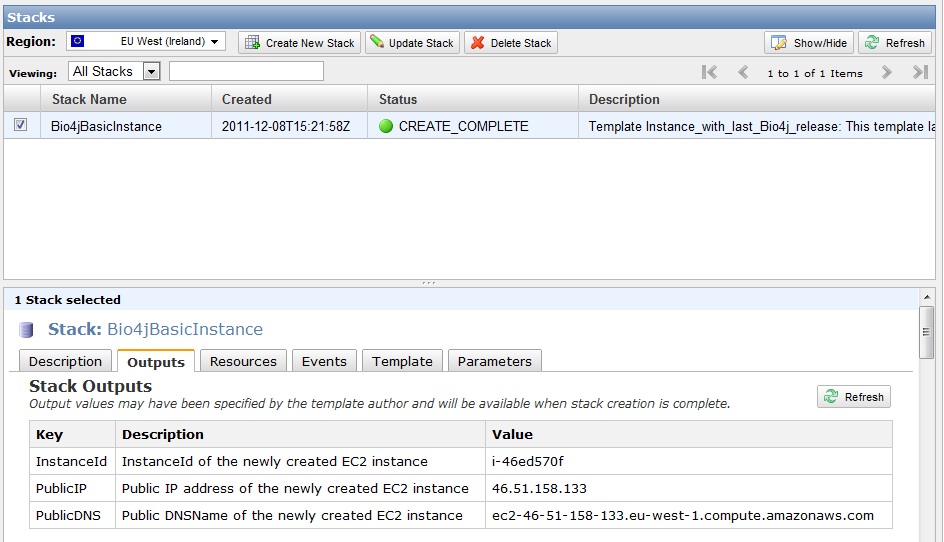
You should be seeing then something like this:
Now you just have to wait for about 30 seconds until after refreshing the stack state changes to green color and says “CREATE_COMPLETE”. Click on the output tab and you will see the IP address you need to connect with SSH to your new instance.
So now you just have to connect to your instance and you should have your fresh backed Bio4j DB under the folder /mnt/bio4j_volume/bio4jdb ;)
Whenever you are done, just select delete stack in the amazon console and don’t worry about terminating your instance or deleting your volume, they will do it for you!
The only thing you have to do is umount the volumes you have attached, it seems that CloudFormation cannot do that for you right now…
After a few months without finding the opportunity to play with Gephi, it was already time to dedicate a lab day to this.
I thought that a good feature would be having the equivalent .gexf file for the current graph representation available at the tab “GoAnnotation Graph Viz”; so that you could play around with it in Gephi adapting it to your specific needs.
Then I got down to work and this is what happened:
First of all I was really happy to see how there was a new version of Gephi (0.8) as well as a good bunch of new (at least for me… :D) layout algorithms plugins available like Parallel Force Atlas, Circular Layout or Layered Layout. So once I have downloaded and installed everything I started to have some fun with it and get to know how filters work, (I haven’t used these ones before).
Even though I got stuck a couple of times trying to figure out how to use some of them, I easily solved these small setbacks thanks to the great support found in the Gephi forums, where they quickly answered my newbie questions, thanks Gephi team!
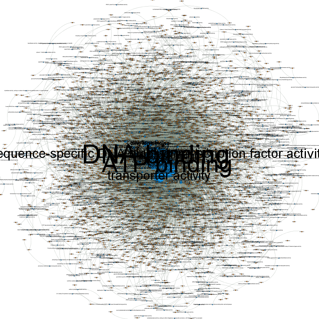
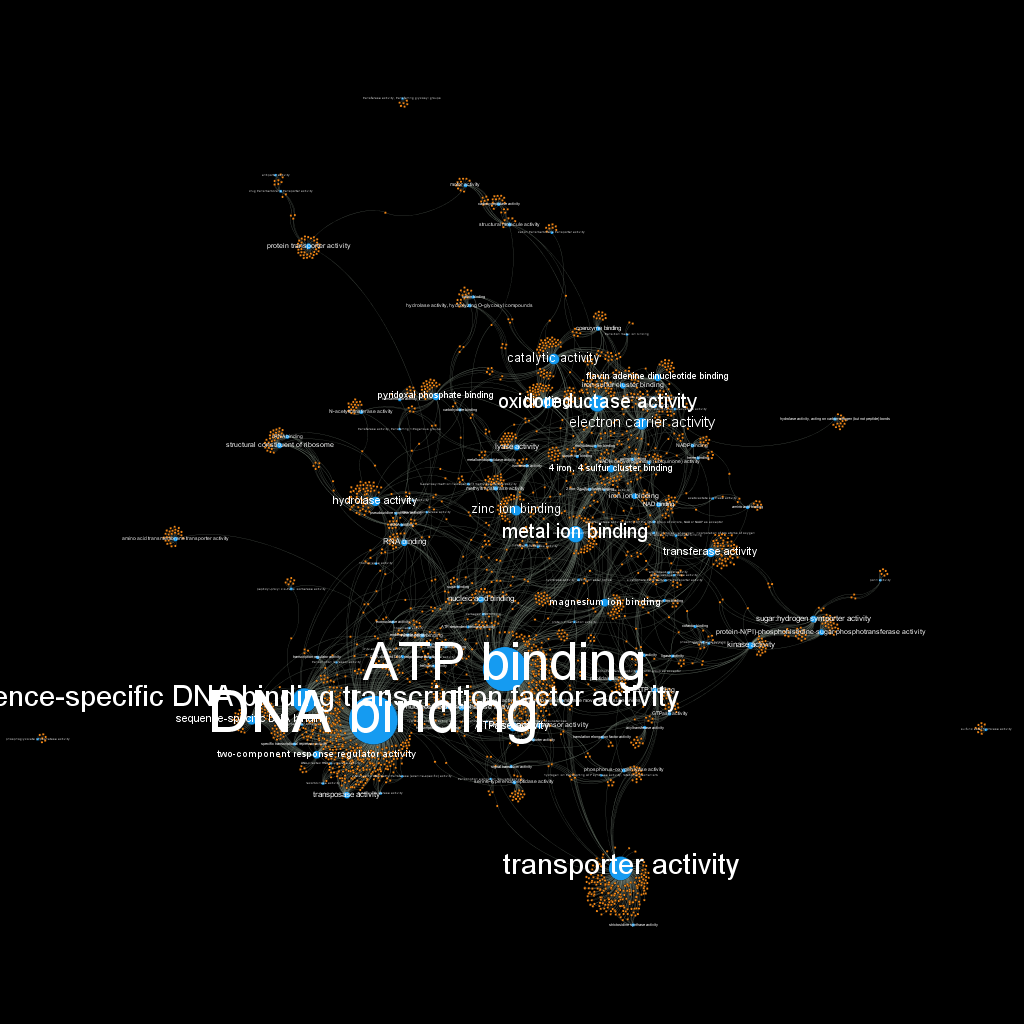
When I first loaded the gexf file in Gephi without applying any kind of filters this is what I got:
As you (maybe) can see, the size of GO term nodes is proportional to the number of proteins they annotate; still it pretty much looks just like a big hair-ball…
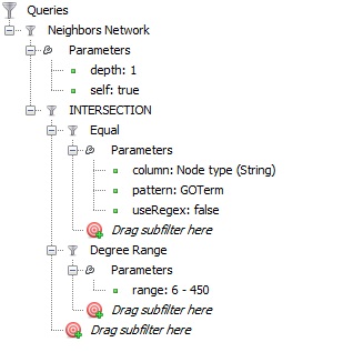
Then I applied the following set of filters:
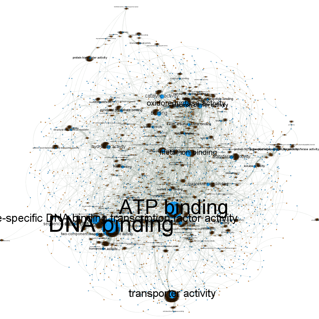
in order to get the GO terms with at least 6 protein annotations plus the proteins which are annotating these terms (their neighborhoods); and this is what it looked like (after applying a Parallel Force Atlas layout algorithm):
I decided then to get rid of the protein labels, since they were way too many and not so useful to be seen; for that I used the option: “Hide nodes/edges labels if not in filtered graph”.
After doing this and applying the black background preview setting, the visualization finally looked pretty decent:
Please go here to check the version exported with Sea Dragon plugin where you can zoom and move around!
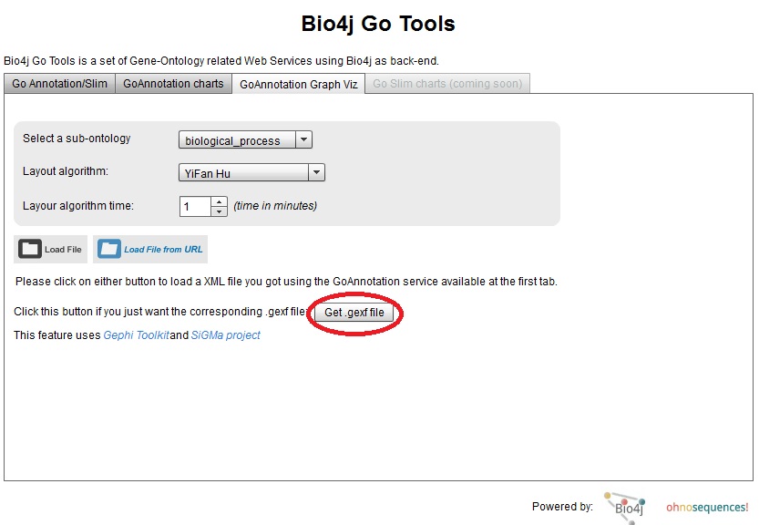
Well, if you like the result (or you don’t but you want to play with this and get a better viz!), I just uploaded a new version of Bio4j GO Tools viewer where you can download the corresponding .gexf file for your GO annotations XML file.
Just press the button highlighted in the screenshot and enter the URL for your GO annotations XML file:
You can use the public EHEC GO annotation results URL I used as a sample for this post:
Amrit
Good to know it. Does it take expression data also. I have expression data with gene name and probe I’d only. Would you mind to suggest whether it work or not for this kind of data. Thank u so much for your help.
Pablo Pareja
Hi Amrit,
There is no restriction for the input data, the only thing is that the tool expects Uniprot accessions as parameters. You would just need to map your gene names to Uniprot accessions using a ID mapping tool such as that available at uniprot website:
http://www.uniprot.org/
(ID mapping tab)
Cheers,
Pablo
Thanksgiving is almost here and we got just in time a lot of special treats for you:
New github organization
All bio4j related repositories are now under the organization bio4j in github.
New wiki(s)
The old wiki hosted at wiki.bio4j.com has been moved to the corresponding Bio4j repository wiki.
More information has been added as well as structuring the previous data. Besides that, new wikis are being created for each bio4j related tools repositories.
NCBI taxonomy
We’re happy to announce the official incorporation of NCBI taxonomy data into Bio4j DB, as well as an index for retrieving NCBI taxons from gene identifiers (GI); so there’s no need anymore to parse that huge gi_taxid_nucl NCBI table in order to achieve that. There’re no changes made to Uniprot taxonomy but you can now navigate to the equivalent NCBI taxon using the relationship NCBITaxonRel.
Reactome terms
We’ve included Reactome terms references included in Uniprot files, so from now on you can retrieve both all terms associated to a specific protein as well as all proteins associated to an specific term.
New EBS snapshot for this release
For those using AWS (or willing to…) there’s a new public EBS snapshot containing the last version of Bio4j DB.
The snapshot details are the following:
Snapshot id: snap-aa5cd3c2
Snapshot region: EU West (Ireland)
Snapshot size: 100 GB
Bio4j DB is under the folder bio4jdb.
In order to use it, just create a Bio4jManager instance and start navigating the graph!
UP 2011 Bio4j presentation
We’re really pleased to announce our presence in this year’s UP 2011 Cloud Computing Conference. The presentation will be held on day 4 Thursday, December 8 2011. Check the agenda for the conference here.